Circle STARKs

Author(s): nguyendinhthang3101, BaoNinh2808

Overview

Scalable and Transparent Arguments of Knowledge (STARK) is a proof system in which a prover generates a proof to convince a verifier of the integrity of a computation. STARK is also a type of Succinct Non-interactive Argument of Knowledge (SNARK). Most other modern SNARKs are pairing-based and rely on elliptic curves, so they must operate over large prime fields to ensure security. However, STARKs are not based on pairings, so their security depends not on the size of the finite field but on the properties of the underlying Interactive Oracle Proof (IOP), specifically the FRI protocol. This means we are not constrained to large prime fields when constructing secure STARKs, opening the door to using smaller, more efficient primes.

For example, several STARKs-based tools and zkVMs have adopted small primes:

• RISC Zero uses the BabyBear prime ($2^{31} - 2^{27} + 1$), a 32-bit prime.
• Pico uses the KoalaBear prime ($2^{31} - 2^{24} + 1$), also 32-bit.
• OlaVM uses the Mini-Goldilocks prime ($2^{64} - 2^{32} + 1$), a 64-bit prime.
• Stone uses the prime $2^{61} + 20 \cdot 2^{32} + 1$, which is 61 bits.

Among all currently used primes, Mersenne31 ($2^{31} - 1$) is the fastest for computation on 32-bit CPUs. It enables extremely efficient multiplication - up to 1.3× faster (HLN23) than BabyBear, which is already the fastest among the commonly used primes in zkVMs and STARKs libraries. For more details, see this blog post by zkSecurity. This makes Mersenne31 an attractive candidate for implementing STARKs.

However, there is a challenge. STARKs rely heavily on two core operations: FFT (Fast Fourier Transform) and FRI (Fast Reed-Solomon IOPP). Both require large multiplicative subgroups of size $2^n$. For primes of the form $c \cdot 2^m + 1$ (where $c$ is an odd integer), we are able to construct multiplicative subgroups of size $2^n$ with $n \le m$. All the primes listed above follow this form, making them naturally compatible with FFT and FRI.

In contrast, Mersenne31 has the form $2^m - 1$ and does not support multiplicative subgroups of size $2^n$ in the same way. To use Mersenne31 as the prime field for STARKs, we need a new mechanism for constructing large multiplicative subgroups and redesigning FFT and FRI to operate over these subgroups.

This is where Circle STARKs come in. Instead of working with traditional 1D subgroups, Circle STARKs operate over 2D points that lie on a circle. The authors of Circle STARKs introduce a novel design for FFT and FRI that works with such 2D multiplicative subgroups, enabling efficient STARKs construction using Mersenne31.

In this report, we introduce the components of Circle STARKs, and explain the intuition behind each component and the underlying mathematics. Our goal is to provide readers who wish to study Circle STARKs with a high-quality reference that covers both the technical details and the design ideas. The structure of this report closely follows the Circle STARKs paper (HLP24) to make it easy to cross-reference.

Flow of Circle STARKs

The diagram below illustrates the overall flow of Circle STARKs (and STARKs in general).

Figure 1: Flow of Circle STARKs

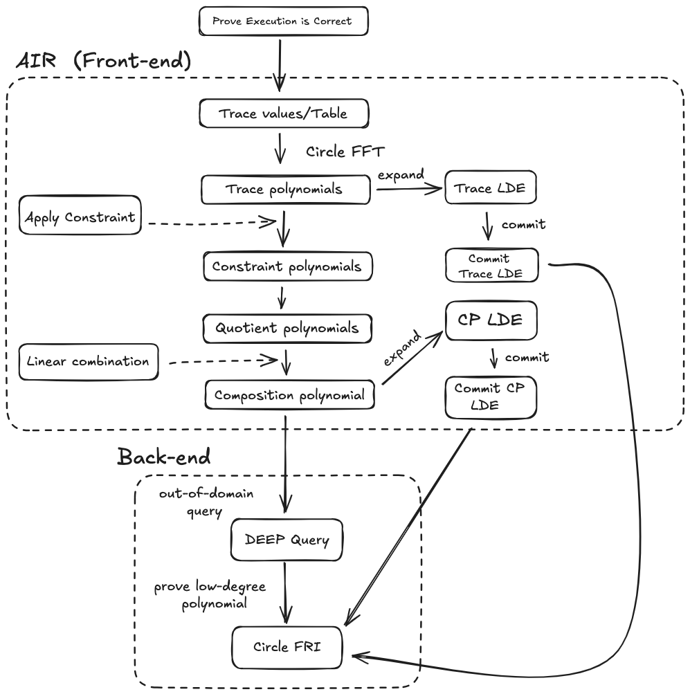
In a Circle STARK (and any STARK), the goal is to generate a proof that convinces the verifier of the integrity of a computation—that is, the correctness of its execution. The first step is to express the computation in Algebraic Intermediate Representation (AIR) so it can be handled by the mathematical back-end.

Front-end: AIR

Within AIR we perform the following steps:

1. Collect Traces – Record the intermediate values that represent the step-by-step execution.
2. Interpolate to Trace Polynomials – Use fast Fourier transform (FFT) to obtain polynomials that encode these traces.
3. Apply Constraints – Impose algebraic constraints capturing the program’s logic, producing Constraint Polynomials.
4. Form the Composition Polynomial – Combine all constraints into a single Composition Polynomial using a polynomial quotient technique and a random linear combination. The constraints are satisfied if and only if this composition polynomial has low degree.
5. Low-Degree Extension and Commitment – Extend the trace and composition polynomials to a larger domain (LDE) and commit to their evaluations with Merkle trees. These commitments serve as the input to the back-end.

Back-end

The back-end’s job is to prove that the composition polynomial derived from the trace is indeed of low degree polynomial. It uses the FRI protocol as the core low-degree test and the DEEP technique to strengthen soundness.

Intuition Behind the Circle STARK Design

Two key operations dominate the STARK/Circle STARK pipeline: FFT and FRI. While FFT could theoretically be replaced by direct Lagrange interpolation, FFT offers far better performance—$O(N \log N)$ versus $O(N^2)$. Both FFT and FRI require working over a multiplicative subgroup of size $2^n$. However, the Mersenne31 prime field does not naturally contain such smooth subgroups.

To use the Mersenne31 prime, the authors introduce a special structure:

• Circle Curve – A 2D curve defined over the Mersenne31 field.
• Circle Group and its cosets – A multiplicative subgroup of the curve with size $2^n$.

Each point on the Circle Curve has two coordinates $(x, y)$. As a result, Circle STARKs operate on 2-dimensional points, unlike standard STARKs, which use 1-dimensional field elements. This requires re-engineering both FFT and FRI to handle the new geometry.

So, the structure of this report:

1. Explore the Circle Curve, the Circle Group, and their cosets.
2. Describe the Circle FFT.
3. Describe the Circle FRI.
4. Integrate all components to present the full protocol.

Circle Curve

In this section, we describe about Circle Curve and explain why Circle Curve build on Mersenne31 prime field has $2^m$ points.

And because it has $2^m$ points then it is ideal for define the group base on this set.

Definition:

Let $\mathbb{F}_p$ be the prime field. The Circle Curve, denoted by $C = C(\mathbb{F}_p)$ is the unit circle over $\mathbb{F}_p$ defined by the equation:

$$C: x^2 + y^2 = 1 \quad \text{with} \quad x,y \in \mathbb{F}_p$$

Or we can write it as the set notion:

$$C = C(\mathbb{F}_p) = \{ (x,y) \in \mathbb{F}_p^2 \quad | \quad x^2 + y^2 = 1 \}$$

Why Circle Curve of Mersenne31 prime field has $2^m$ points?

The Lemma 1 in Circle STARKs paper say that the Circle Curve of the finite field $\mathbb{F}_p$ has total |$\mathbb{F}_p$| + 1 points. Then if our finite field is Mersenne31 prime field with $p=2^m -1$, the total points is $(2^m - 1) + 1 = 2^m$.

Proof of Lemma 1:

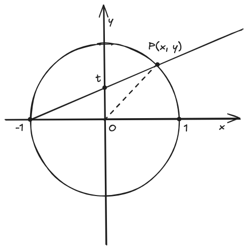
$\forall P(x,y) \in C(\mathbb{F}_p)$ we draw a line to $(-1, 0)$. This line intersects the $y$-axis (projective line) at $t$ with $t = \frac{y}{x+1}$ with $x,y \in \mathbb{F}_p$ (see Figure 2).

• For all $(x,y) \neq (-1,0)$ we can calculate $t \in \mathbb{F}_p$. Each $(x,y) \neq (-1,0)$ is correspond to one value $t \in F_{p}$. We have total |$\mathbb{F}_p$| possible values for $t$ mean there are total |$\mathbb{F}_p$| valid points $(x,y) \neq (-1,0)$.
• When $(x,y) = (-1,0)$, $t \to \infty$.

So that in total we have $(|\mathbb{F}_p|+1)$ valid points in $C(\mathbb{F}_p)$

Figure 2: Stereographic projection

Circle Group

Circle Group is Circle Curve with operation $\bullet$ defined as:

$$(x_1, y_1) \bullet (x_2, y_2) = (x_1x_2 - y_1y_2, x_1y_2 + x_2y_1)$$

This definition of group operation satisfies group axioms:

• Identity : The identity/neutral element is $(1,0)$
  • Since $(x,y) \bullet (1,0) = (x.1 - y.0, x.0 + y.1) = (x,y)$
• Inverse : For every element $(x,y) \in C$, the inverse of an element is $J(x,y) = (x, -y) \in C$
  • Since $(x,y) \bullet (x,-y) = (x^2 + y^2, x.y - x.y) = (1,0)$
• Associativity : For all $(x_1, y_1), (x_2, y_2), (x_3, y_3) \in C$ : $[(x_1, y_1) \bullet (x_2, y_2)] \bullet (x_3, y_3) = (x_1, y_1) \bullet [(x_2, y_2) \bullet (x_3, y_3)]$
• Closure : For all $(x_1, y_1), (x_2, y_2) \in C$ : $(x_1, y_1) \bullet (x_2, y_2)$ is an element of $C$
  • Since from $x_1^2 + y_1^2 = 1$ and $x_2^2 + y_2^2 = 1$ we have $(x_1x_2 - y_1y_2)^2 + (x_1y_2 + x_2y_1)^2 = 1$.

With $\mathbb{F}_p$ is Mersenne31 prime field, we have $(C(\mathbb{F}_p), \bullet)$ is group with $2^m$ elements. Now we need to prove this is cyclic multiplicative group.

Proof that the Circle Group Is a Cyclic Multiplicative Group

Consider the Circle Group

$$C(\mathbb{F}_p) \;=\; \bigl\{(x,y)\in \mathbb{F}_p^2 \;\big|\; x^2 + y^2 = 1\bigr\}$$

equipped with the operation

$$(x_1,y_1)\,\bullet\,(x_2,y_2) \;=\; \bigl(x_1x_2 - y_1y_2,\; x_1y_2 + x_2y_1\bigr).$$

1. Relation to a “Complex” Group

Define the set

$$\mathbb{S} \;=\; \bigl\{x + i y \in \mathbb{F}_{p^2}\;\big|\; \; x^2 + y^2 = 1 \bigr\},$$

where $i$ is a formal symbol with $i^2 = -1$.

Note that $\mathbb{F}_{p^2}$ is different with $\mathbb{F}_p^2$.

Equip $\mathbb{S}$ with the multiplication

$$(x_1 + i y_1)\,\bullet\,(x_2 + i y_2) \;=\; (x_1 x_2 - y_1 y_2) + i (x_1 y_2 + x_2 y_1).$$

This is exactly the usual multiplication of complex numbers, but carried out inside the finite field $\mathbb{F}_p$.

The map

$$\varphi: C(\mathbb{F}_p) \longrightarrow \mathbb{S}, \qquad \varphi(x,y) = x + i y$$

is a group isomorphism:

• It is bijective because every $x+iy$ with $x^2 + y^2 = 1$ corresponds uniquely to a pair $(x,y)$ with the same relation.

• It preserves the operation because

  $$\varphi\bigl((x_1,y_1)\bullet(x_2,y_2)\bigr) = (x_1x_2 - y_1y_2) + i(x_1 y_2 + x_2 y_1) = \varphi(x_1,y_1)\bullet \varphi(x_2,y_2).$$

Hence proving that $(\mathbb{S},\bullet)$ is cyclic immediately shows that $(C(\mathbb{F}_p),\bullet)$ is cyclic.

2. Embedding $\mathbb{S}$ in a Finite-Field Extension

Write $\mathbb{F}_{p^2} = \mathbb{F}_p[i]$ where $i^2=-1$. The multiplicative group $\mathbb{F}_{p^2}^\times$ is cyclic of order $p^2 - 1$. (let prove it yourself)

For any $\alpha = x + i y \in \mathbb{F}_{p^2}$, its norm is

$$N(\alpha) = \alpha \cdot \overline{\alpha} = (x + i y)(x - i y) = x^2 + y^2.$$

Thus

$$\mathbb{S} \;=\; \{\alpha \in \mathbb{F}_{p^2}^\times \mid N(\alpha) = 1\}.$$

This is precisely the kernel of the norm map

$$N : \mathbb{F}_{p^2}^\times \longrightarrow \mathbb{F}_p^\times.$$

3. Size and Cyclicity of $\mathbb{S}$

The norm map is a surjective group homomorphism. By the First Isomorphism Theorem,

$$\bigl|\ker N\bigr| = \frac{|\mathbb{F}_{p^2}^\times|}{|\mathbb{F}_p^\times|} = \frac{p^2 - 1}{p - 1} = p + 1.$$

Thus $|\mathbb{S}| = p + 1$. (We can also use this result to prove that the number of elements in Circle Group is $p+1 = 2^m$).

It is a standard result that every subgroup of a cyclic group is cyclic. Since $\mathbb{F}_{p^2}^\times$ is cyclic and $\mathbb{S}$ is a subgroup of size $p+1$, it follows that $\mathbb{S}$ is itself cyclic. And because the operation define in $\mathbb{S}$ is multiplication ($\bullet$) so $\mathbb{S}$ is multiplicative subgroup.

4. Conclusion

Because $C(\mathbb{F}_p)$ is isomorphic to $\mathbb{S}$, we conclude:

$$\boxed{\ (C(\mathbb{F}_p),\bullet) \ \text{is a cyclic multiplicative group of order } p + 1. \ }$$

Other operations define on Circle Group:

Square map

Square map is the squaring for a point defined as

$$\pi(x, y) = (x,y)\bullet(x,y) = (x^2 - y^2, 2xy)=(2x^2-1, 2xy)$$

Inverse

The inverse is define as:

$$J(x,y) = (x,-y)$$

If we square $(x,y)$ and its inverse $(x,-y)$, we obtain the same $x$-coordinate $2x^2 - 1$, while the $y$-coordinate is the inverse. This means that if we visualize the Circle Group as a circle in 2D, then $\pi(x,y)$ and $\pi(x,-y)$ are mirror images across the $x$-axis.

Circle Domain

In this section, we introduce the actual domain used in Circle STARKs, called the Standard Position Coset. This domain is built from a Twin-coset, which in turn is formed from a coset of the Circle Group.

You can think of our progression so far as follows: first we explored the Circle Curve, then we built the Circle Group on it, next we used that group to create the Twin-coset, and finally we formed the Standard Position Coset - the real domain used in Circle STARKs.

For readers who are not familiar with the term coset, it is simply a group that has been shifted by multiplying or adding a constant. For example, let our group be

$$\mathbb{G} = \{1, 3, 5, 7\}.$$

A coset of $\mathbb{G}$ can be obtained by multiplying every element by $2$:

$$\mathbb{C} = 2 \cdot \mathbb{G} = \{2, 6, 10, 14\},$$

assuming the group operation in $\mathbb{G}$ is multiplication.

Twin-coset

It is natural to choose a cyclic multiplicative subgroup $G_n$ of size $2^n$ (with $n \le m$) from a cyclic multiplicative group $C(\mathbb{F}_p)$ of size $2^m$.

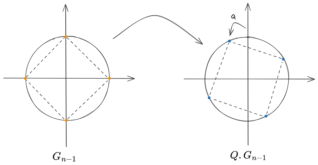
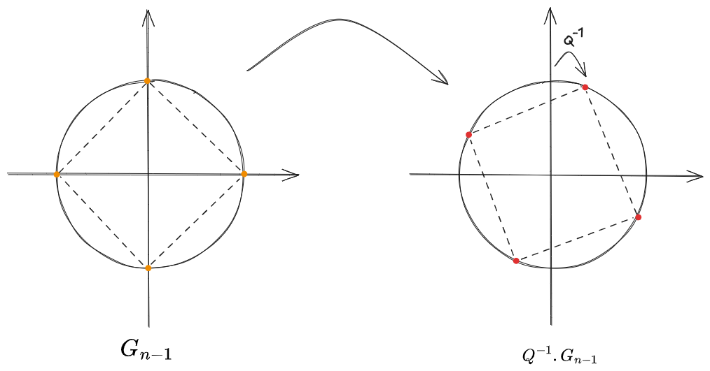
Let $G_{n-1}$ be a cyclic subgroup of $C(\mathbb{F}_p)$ of size $|G_{n-1}| = 2^{n-1}, n \geq 1$. We pick a point $Q \in C(\mathbb{F}_p)$, which must not be the identity element or have order two $(Q^2=1)$. So we can construct 2 cosets $Q \bullet G_{n-1}$ and $Q^{-1} \bullet G_{n-1}$ of subgroup $G_{n-1}$:

1. Rotation by $Q$: Multiplication of $G_{n-1}$ by $Q$ corresponds to rotating $G_{n-1}$ in the counterclockwise direction. This is visualized as the rotated blue points representing $Q \bullet G_{n-1}$

Figure 3: Construct coset by rotating Q

2. Rotation by $Q^{-1}$: Multiplication of $G_{n-1}$ by $Q^{-1}$ corresponds to rotating $G_{n-1}$ in the clockwise direction. This is visualized as the rotated red points representing $Q^{-1} \bullet G_{n-1}$

Figure 4: Construct coset by rotating inverse Q

If $Q \bullet G_{n-1} \cap Q^{-1} \bullet G_{n-1} = \varnothing$ (i.e., two coset does not have any shared elements) then we call $D = Q \bullet G_{n-1} \cup Q^{-1} \bullet G_{n-1}$ (the unite of 2 cosets) is "Twin-Coset" of size $2^n$.

Figure 5: Construct twin-coset

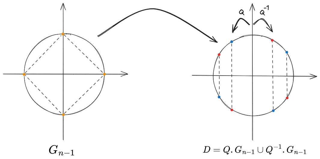
This set is called a Twin-Coset because the two cosets are mirror images across the $x$-axis. Sometimes they can also be mirrored across the $y$-axis, but not always. When that occurs, we call it a Standard Position Coset.

Exlain why Q must not be the identity element or have order two

If we know $Q$ that $Q \bullet G_{n-1} = Q^{-1} \bullet G_{n-1}$ and multiply by $Q$ of both sides we have $Q^2 \bullet G_{n-1} = G_{n-1} \implies Q^2 = (1,0)$ or $Q = (1, 0)$, which is why $Q$ can't be the identity element or have order two.

Figure 6: Choose Q = (1,0) or Q have order two could lead to constructing bad coset

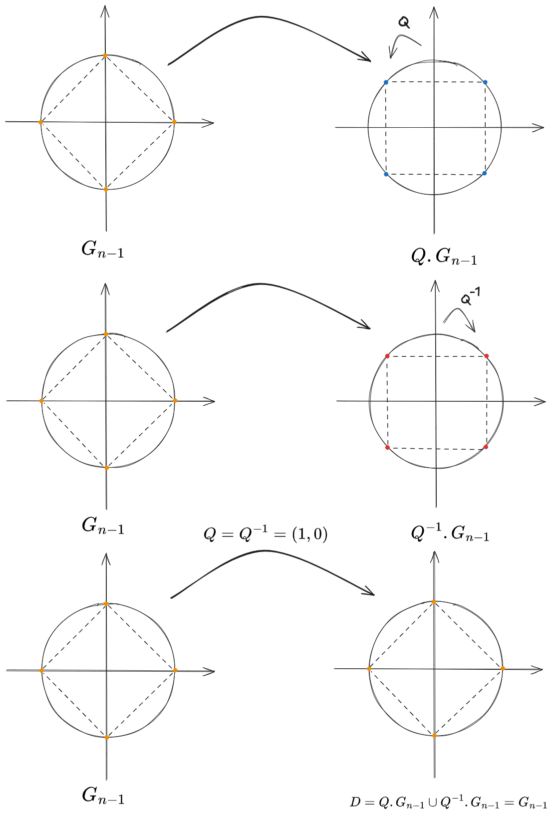
Inverse map $J$ of the point from one coset is the point of other which mirrors by $x$-axis. $\forall g \in Q \bullet G_{n-1}: J(g) \in Q^{-1} \bullet G_{n-1}$. That's why it's called "Twin-coset"

Standard position coset

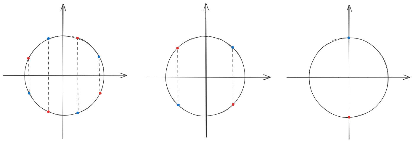
If twin-coset of $G_{n-1}$ is coset of $G_n$ then it is called Standard Position Coset. This mean: If $D = Q \bullet G_{n-1} \cup Q^{-1} \bullet G_{n-1}$ is a coset of $G_n$ then $D$ is standard position coset. In standard position position coset, each point is equidistant to nearby (Figure 7). In Circle STARK, both trace domain and evaluation domain are standard position coset. To construct standard position coset of size $2^n$, the order of $Q$ is $2^{n+1}$. (Proposition 1 in paper Circle STARKs HLP24)

Figure 7: Standard position cosets of size 2^3, 2^2 and 2^1

Circle FFT

In the STARK protocol, the computation trace consists of values that lie in a multiplicative subgroup. We interpolate these values to obtain a polynomial that represents the trace. STARKs use the Fast Fourier Transform (FFT) to perform this interpolation efficiently.

Circle STARKs follow the same idea, but the multiplicative subgroup is replaced by the Circle Domain, which contains 2-dimensional points rather than the 1-dimensional points of a finite field multiplicative subgroup. Circle FFT is a specialized Fast Fourier Transform designed for this Circle Domain (Standard Position Coset).

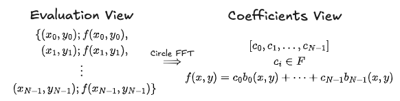
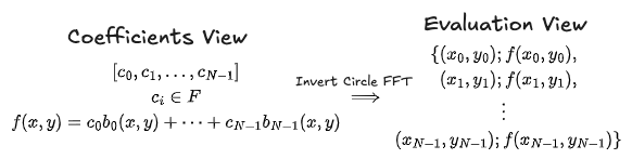
Given the evaluations of a polynomial (the evaluation view) over a multiplicative subgroup $D_n$ of size $N = 2^n$, the goal of the Circle FFT is to compute the coefficients $(c_0, c_1, \ldots, c_{N-1})$ (the coefficient view) of a polynomial of degree $< N$ (see Figure 8). The functions $b_0(x,y), \ldots, b_{N-1}(x,y)$ form the FFT basis, which will be explained later.

Figure 8: Visualization of Circle FFT

Vanishing Polynomial

To understand the Circle FFT, first we need to understand one of its tool named Vanishing Polynomial.

A vanishing polynomial (of a given set) is any non-zero polynomial that evaluate to zero at every point of a given set. In STARK constructions, program constraints are expressed as polynomials evaluated over the computation trace; a valid execution makes those polynomials vanish at every point of the trace domain. Therefore each constraint polynomial must be a multiple of the trace-domain’s vanishing polynomial. Since Circle STARKs use a Standard Position Coset as their trace domain, we focus on the vanishing polynomials that vanish on these Standard Position Coset. But Standard Position Coset is a special case of twin-coset, so that we start by find the vanishing polynomial of twin-coset.

Vanishing Polynomial in Twin-Coset

Generally, applying the squaring map $n-1$ times to a twin-coset $D$ of size $N = 2^n$ give a twin-coset of size 2, which is defined as follow:

$$\pi^{n-1}(D) = \{(x_D, y_D),(x_D, -y_D)\}$$

After we project the points onto the $x$-axis, they turn out $x$-coordinate $x_D$:

$$\pi_x \circ \pi^{n-1}(D) = x_D$$

where $\pi_x$ is the projection onto $x$-axis. The vanishing polynomial over the twin-coset $D$ can be defined as:

$$v_D(x,y) = \pi_x \circ \pi^{n-1}(x, y) - x_D \quad \forall x,y \in D$$

Vanishing Polynomial in Standard Position Coset

In the special case of standard position coset, after applying square map $n-1$ times on D, the final pair of points lie on $y$-axis $\implies x_D = 0$. Thus, The vanishing polynomial over standard position coset $D$ is

$$v_D(x,y) = v_n(x,y) = \pi_x \circ \pi^{n-1}(x, y)$$

In the square map, the $x$-coordinate of the result does not related to the value of $y$ of the input. In vanishing polynomial, as the end we project the point on $x$-axis (i.e., does not concern about the $y$ value). So that, in vanishing polynomial we can only concern about the $x$ value.

$$v_n(x,y) = v_n(x) \quad \text{because} \quad \pi_x \circ \pi^{n-1}(x, y) = \pi_x \circ \pi^{n-1}(x)$$

where the square map on only $x$-coordinate is define by:

$$\pi(x) = 2x^2 - 1$$

From now, when we say about vanishing polynomial over Standard Position Coset, we see it as a univariate polynomial:

$$v_n(x) = \pi_x \circ \pi^{n-1}(x) = \pi^{n-1}(x)$$

Bivariate Polynomial Space

Let's $\mathcal{L}_{N}(F)$ denote for the space of bivariate polynnomials over circle curve

$$\mathcal{L}_{N}(F) = \{ p(x,y) \in F[x,y]/(x^2 + y^2 -1) : deg(p) \leq \frac{N}{2} \}$$

where:

• $F$ is the (extension) field that we're working on.
• The bivariate polynomials is modulo by $x^2 + y^2 -1$
• The max degree of bivariate polynomial is $\frac{N}{2}$. This means for each term $x^a.y^b$ it satisfies $a + b \leq \frac{N}{2}$.

Because of $x^2 + y^2 -1 = 0$, then we can substitute all the term $y^2$ in bivariate polynomial by $1 - x^2$ and reduce $p(x,y)$ to the form

$$p(x,y) = p_0(x) + y \cdot p_1(x)$$

Since $p(x,y)$ has the max degree $\leq \frac{N}{2}$. This lead to $p_0$ has the degree $\leq \frac{N}{2}$ and $p_1$ has the degree $\leq \frac{N}{2}-1$. So we can implies that the space $\mathcal{L}_{N}(F)$ is spanned by the following basis:

$$1,x,x^2,...x^{\frac{N}{2}},y,yx,yx^2,...,yx^{\frac{N}{2}-1}$$

There are total $N+1$ basises, mean the bivariate polynomial space $\mathcal{L}_{N}(F)$ has $N+1$ dimension.

FFT Space

FFT Space is where the bivariate polynomial interpolate from Circle FFT belong to.

The FFT space $\mathcal{L}'_{N}(F)$ of the Circle Curve is a set of polynomials with the formula:

$$\mathcal{L}'_{N}(F)=\{p(x,y) \in F[x,y] \ | \ p(x,y) = \displaystyle\sum_{j=0}^{2^{n}-1}c_{j}b_{j}^{(n)}(x,y) \}$$

where $b^{(n)}_j$ is the FFT basis defined at index $j$ as below:

$$b_{j}^{(n)}(x, y) = y^{j_0} \cdot v_1(x)^{j_1} \cdot v_2(x)^{j_2} \dots v_n(x)^{j_{n-1}}$$

with $j = \overline{j_{n-1} \dots j_2 j_1 j_0}$ is the binary representation and $0 \leq j \leq 2^{n}-1$

In FFT basis formulae, each $v_k(x)$ (for $1 \leq k \leq n-1$) is the vanishing polynomial of the standard position coset of size $2^k$:

$$v_k(x) = \pi^{k-1}(x), \quad 1 \leq k \leq n-1$$

There are total $2^n$ FFT basises, mean FFT Space $\mathcal{L}'_{N}(F)$ has $2^n$ dimension.

Dimension Gap

Set $N=2^n$, the basis $b_{j}^{(n)}(x, y)$ has a total $N=2^n$ elements and we can implies that the dimension of FFT Space $\mathcal{L}'_{N}(F)$ is $N$. However, the space of bivariate polynnomials over circle curve $\mathcal{L}_{N}(F)$ has the dimension $N+1$. Because $dim(\mathcal{L}'_{N}(F)) < dim(\mathcal{L}_{N}(F))$, FFT Space does not contain all bivariate polynomial in $\mathcal{L}_{N}(F)$. We will investigate about the missing dimension in FFT Space when compare to Bivaritate Polynomial Space.

Since the highest degree of $x$ in FFT basis is $\frac{N}{2} -1$ (when $j_1 \to j_{n-1} = 1$. The space $\mathcal{L}'_{N}(F)$ can be expressed as:

$$\mathcal{L}'_{N}(F) = F[x]^{\leq \frac{N}{2}-1} + y.F[x]^{\leq \frac{N}{2}-1}$$

where $F[x]^{\leq \frac{N}{2}-1}$ represents polynomials of degree at most $\frac{N}{2}-1$ with coefficients in $F$.

Similarly, we can represent the space $\mathcal{L}_{N}(F)$ as:

$$\mathcal{L}_{N}(F) = F[x]^{\leq \frac{N}{2}} + y.F[x]^{\leq \frac{N}{2}-1}$$

Because the space $\mathcal{L}'_{N}(F)$ does not include the monomial $x^{\frac{N}{2}}$ which is in $\mathcal{L}_{N}(F)$. So that:

$$\mathcal{L}_{N}(F) = \mathcal{L}'_{N}(F) \ \ + \ \ \langle x^{N/2} \rangle$$

Since the space spanned by $x^{\frac{N}{2}}$ is same as the space spanned by the vanishing polynomial $v_n(x)$ which has degree as $deg(v_n)=2^{n-1}=\frac{N}{2}$. We can also write:

$$\mathcal{L}_{N}(F) = \mathcal{L}'_{N}(F) \ \ + \ \ \langle v_n \rangle$$

The idea of Dimension Gap is useful in Circle FRI.

Circle FFT Algorithm

Sequence of Domain used in Circle FFT

With $D_n$ is the Twin-coset with size $2^n$ (Standard Position Coset is special case of Twin-coset):

$$D_n = Q \bullet G_{n-1} \cup Q^{-1} \bullet G_{n-1}$$

where $G_{n-1}$ has the size of $2^{n-1}$ and $Q \neq Q^{-1}$.

We define 2 type of maps as follow:

1. Quotient map $\phi_J$: This map sends each point in $D_n$ to an element of the quotient set $D_n/J$:

$$\begin{align*} \phi_J: D_n &\longrightarrow D_n/J \\ P &\longmapsto \{P,\ J(P)\} \end{align*}$$

where $J$ denotes the inversion map $J(P) = -P$. Quotient map $\phi_J$ maps two distinct points $P$ and $J(P)$ from $D_n$ to a single element in $D_n/J$ (this element is $\{P,\ J(P)\}$). $D_n/J$ is a set of all classes is separated by $J$. We can define a class like this:

$$\text{class}_{P} = \{X \in D_n \ | \ J^{t}(X) = P, \ t \in \mathbb{N}^{*}\}$$

This class exactly includes 2 elements (correspond to $t$ odd and even):

$$\text{class}_{P} = \{P, \ J(P)\}$$

This is 2-to-1 map, bacause it maps 2 elements $P$ and $J(P)$ to 1 class $\{P, \ J(P)\}$. The map $\phi_J$ is equal to projection map $\pi_x$ that projects the points $(x, \pm \ y)$ to the same $x$-coordinate:

$$\pi_x((x, y)) = \pi_x((x, - y)) = x$$

We use the notion $S_n$ for the quotient $D_n/J$ when only consider $x$-coordinate:

$$\pi_x: D_n \longrightarrow S_n$$

2. Squaring map $\pi$: This map was introduced in previous section circle curve. When applying it to the twin-coset $D_n$ of size $2^n$. It generates a smaller twin-coset $D_{n-1}$ which also halves the size of $D_n$:

$$\begin{align*} \pi: D_n &\longrightarrow D_{n-1} \\ (x, y) &\longmapsto (2x^2-1, 2xy) \end{align*}$$

From these 2 maps we define above, we build the the sequence of 2-to-1 map in Figure 9.

Figure 9: Sequence of 2-to-1 map

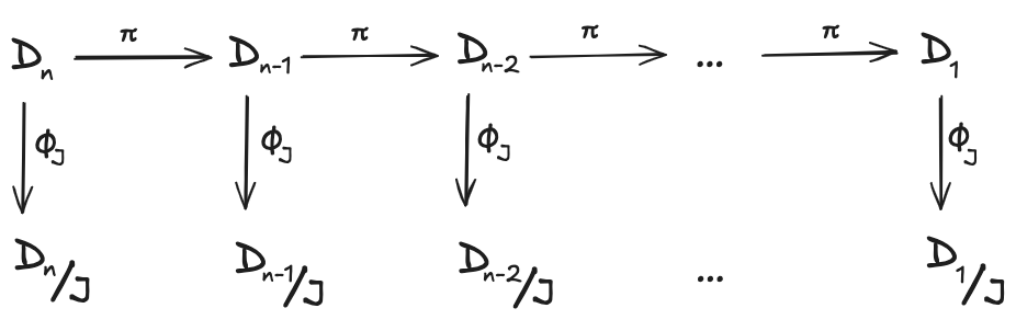
Because $J$ and is commute:

$$J(\pi(P)) = \pi(J(P))$$

Then the result of applying $\pi$ map then $\phi_J$ map is equal to applying $\phi_J$ map then $\pi$ map. So we have:

Figure 10: Sequence of 2-to-1 map

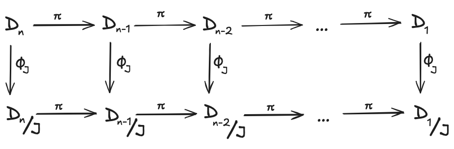
Because each class in $D_j/J$ have the form $\{P, J(P)\}$. So we can use only $x$-coordinate to represent the class of $D_j/J$. So in Circle STARKs, they use the domain $S_j$ substitute for $D_j/J$

The sequence of domains use in Circle FFT is shown as Figure 11, 12, 13 below:

Figure 11: Sequence of domain used in Circle FFT

Figure 12: Sequence of domain used in Circle FFT

Figure 13: Sequence of domain used in Circle FFT without projection on x-axis

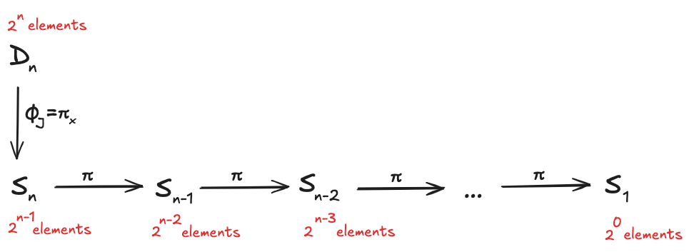
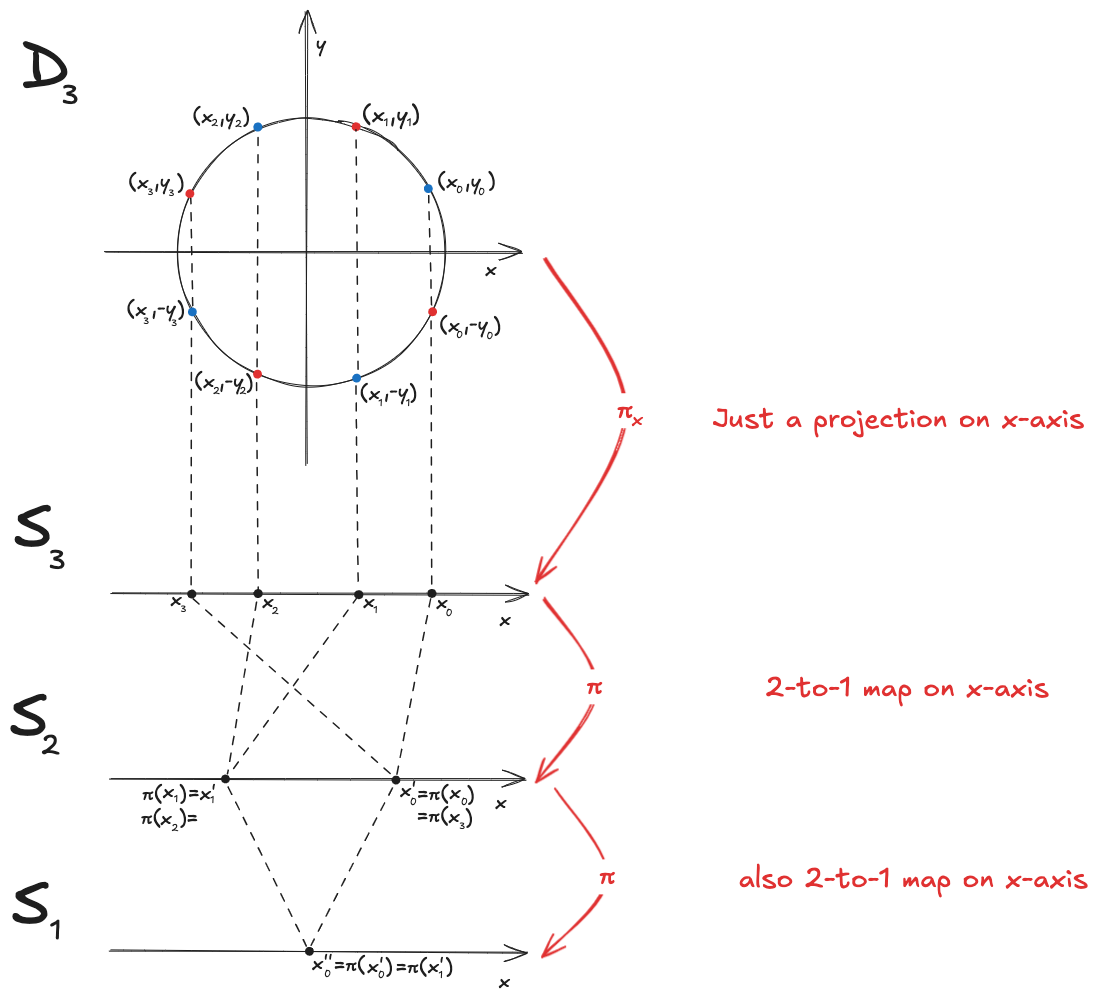
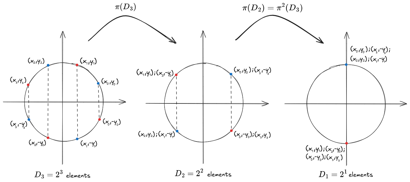
In Circle FFT, we use both projection map $\pi_x$ and $\pi$ to construct of the sequence of domains. Since the map $\pi_x$ and $\pi$ commute:

$$\pi_x \circ \pi(D_n) = \pi \circ \pi_x(D_n)$$

Algorithm

Circle FFT follows the same divide-and-conquer strategy as the normal FFT algorithm. The bivariate polynomial is first decomposed into polynomials with lower degree. We then recursively compute the coefficients of these smaller polynomials and finally combine them to compute the coefficients of the original polynomial. The Circle FFT algorithm has many rounds, we describe each round as follow:

Round 1: We have the Evaluation View:

$$\begin{array}{c|c} (x,y) & (x_0,y_0) & \cdots & (x_{\frac{N}{2}-1}, y_{\frac{N}{2}-1}) & (x_0, -y_0)\\ \hline f(x,y) & f(x_0,y_0) & \cdots & f(x_{\frac{N}{2}-1}, y_{\frac{N}{2}-1}) & f(x_0, -y_0) \end{array}$$

with $f(x_i, y_i) \in F$. ($F$ can be Mersenne31 field or the extension fiel of it, Circle FFT can work in both cases). We need to compute $[c_0,...,c_{N-1}]$ (Coefficient view) with $c_i \in F$

First, We decomposes: $f(x,y) = f_0(x) + yf_1(x)$ with $\begin{cases}f_0 = [c_0, c_2, ...] \\ f_1 = [c_1,c_3,...]\end{cases}$ Because of structure of FFT basis: $b_j(x,y) = y^{j_0}v_1(x)^{j_1}\cdots v_{n-1}(x)^{j_{n-1}}$. So that

$$\begin{cases}f_0(x) = \frac{f(x,y) + f(x,-y)}{2} \\ f_1(x) = \frac{f(x,y) - f(x,-y)}{2y}\end{cases}$$

$\implies$ We can calculate evaluation view of $f_0(x)$ and $f_1(x)$ from evaluation view of $f(x,y)$

Round 2: (just consider $f_0(x)$, similar for $f_1(x)$)

We have the Evaluation View of $f_0(x)$:

$$\begin{array}{c|c} x & x_0 & \cdots & x_{\frac{N}{2}-1}\\ \hline f(x) & f(x_0) & \cdots & f(x_{\frac{N}{2}-1}) \end{array}$$

We need to compute $[c_0, c_2, \cdots,c_{N-2}]$ (Coefficient view) with $c_i \in F$

$$f_0(x) = c_0b_0(x) + c_2b_2(x) + \cdots + c_{N-2}b_{N-2}(x)$$

We can write $f_0(x) = f_{00}(\pi(x)) + xf_{01}(\pi(x))$ with $\begin{cases}f_{00} = [c_0,c_4,c_8,\cdots,c_{N-4}]\\f_{01} = [c_2,c_6,c_{10}, \cdots,c_{N-2}]\end{cases}$

Because with $j \ \vdots \ 4$, we write $j = 4k = \overline{j_{n-1}\cdots j_{2}00}$

$$b_j(x) = v_2(x)^{j_2} \cdots v_{n-1}(x)^{j_{n-1}}$$

with $j \ \vdots \ 2$ but $j \ \not \vdots 4$ we write $j = \overline{j_{n-1} \cdots j_{2}10}$

$$b_j(x) = v_1(x)v_2(x)^{j_2} \cdots v_{n-1}(x)^{j_{n-1}}$$

So we can represent $b_j=v_1(x)b_{j-2}(x)=xb_{j-2}(x) \ \forall j \not \vdots 4$ Thus, we write $f_0(x)$ like

$$f_0(x) = \bigg( c_0b_0(x) + c_4b_4(x) + \cdots + c_{N-4}b_{N-4}(x) \bigg) + x \bigg( c_2b_0(x) + c_6b_4(x) + \cdots + c_{N-4}b_{N-4}(x) \bigg)$$

We have the special feature of vanishing polynomial

$$\begin{cases} v_1(x) = x \\ v_2(x) = 2v_1(x)^2 - 1 = 2x^2-1 \\ v_3(x) = 2v_2(x)^2 - 1 \\ v_4(x) = 2v_3(x)^2 - 1 \end{cases} \implies \begin{cases} v_1(\pi(x)) = \pi(x) = 2x^2-1 = v_2(x)\\ v_2(\pi(x)) = 2v_1(\pi(x))^2 - 1 = 2v_2(x)^2 - 1 = v_3(x) \\ v_3(\pi(x)) = 2v_3(x)^2 - 1 = v_4(x)\\ v_4(\pi(x)) = 2v_4(x)^2 - 1 = v_5(x) \end{cases}$$

Generally we have : $v_j(\pi(x)) = v_{j+1}(x)$

So that, for $j \ \vdots \ 4$:

$$\begin{align*} b_j &= v_2(x)^{j_2} \cdots v_{n-1}(x)^{j_{n-1}} \\ &= v_1(\pi(x))^{j_2} \cdots v_{n-2}(\pi(x))^{j_{n-1}} v_{n-1}(\pi(x))^0 \\ &= b_{j/2}(\pi(x)) \end{align*}$$

with $j/2 = \overline{0j_{n-1} \cdots j_20}$

We can rewrite $f_0(x)$ in another way:

$$\begin{align*} f_0(x) &= \bigg( c_0b_0(\pi(x)) + c_4b_2(\pi(x)) + \cdots + c_{N-4}b_{\frac{N}{2}-1}(\pi(x)) \bigg) \\ &+ x\bigg(c_2b_0(\pi(x)) + c_6b_2(\pi(x)) + \cdots c_{N-2}b_{\frac{N}{2}-1}(\pi(x))\bigg) \\ &= f_{00}(\pi(x)) + xf_{01}(\pi(x)) \end{align*}$$

with $\begin{cases}f_{00}(z) = c_0b_0(z) + c_4b_2(z) + \cdots \\ f_{01}(z) = c_2b_0(z) + c_6b_2(z) + \cdots \end{cases}$

The problem now is to find coefficients $[c_0, c_4, \cdots, c_{N-4}]$ correspond to basis $b_0, b_2, b_4, \cdots, b_{\frac{N}{2}-1}$ and $[c_2, c_6, \cdots, c_{N-2}]$ correspond to basis $b_0, b_2, b_4, \cdots, b_{\frac{N}{2}-1}$

$\implies$ The original problem of finding $[c_0, c_2, \cdots, c_{N-2}]$ correspond to $[b_0, \cdots, b_{N-2}]$ is split into 2 subproblems with identical structure but the number of basis is half down

From the evaluation view of $f_0(x)$ we can compute evaluation view of $f_{00}(z)$ and $f_{01}(z), \ z = \pi(x)$ with $\begin{cases}f_{00}(\pi(x)) = \frac{f_0(x) + f_0(-x)}{2} \\ f_{01}(\pi(x)) = \frac{f_0(x) - f_0(-x)}{2x}\end{cases}$

Round 3: (just consider $f_{00}(\pi(x))$, similar for $f_{01}(\pi(x))$)

We have:

$$\begin{array}{c|c} \pi(x) & \pi(x_0) & \cdots & \pi(x_{\frac{N}{4}-1})\\ \hline f_{00}(\pi(x)) & f_{00}(\pi(x_0)) & \cdots & f_{00}(\pi(x_{\frac{N}{4}-1})) \end{array}$$

The index of $x$ is $\frac{N}{4}-1$ because $\pi$ is 2-to-1 map (see the visualization)

Now, we meet the same problem as in Round 2. So that we apply the same technique here. We don't verbose here.

Round 4: Similar to Round 2, 3 ... Round n+1: As round n+1, our evaluation view has 1 element left.

$$\begin{array}{c|c} \pi^{n-1}(x) & \pi^{n-1}(x_0)\\ \hline f_{0\cdots 0}(\pi^{n-1}(x)) & f_{0\cdots 0}(\pi^{n-1}(x_{0})) \end{array}$$

We want to find the coefficient view $[c_0]$. This mean:

$$f_{0\cdots 0}(z) = c_0, \quad c_0 \text{ is coefficient at } z^0$$

$\implies c_0 = f_{0 \cdots 0}(\pi^{n-1}(x_0))$

Similar:

$$\begin{align*} c_1 &= f_{0 \cdots 1}(\pi^{n-1}(x_0)) \\ c_2 &= f_{00 \cdots 10}(\pi^{n-1}(x_0)) \\ \vdots \\ c_{N-1} &= f_{1 \cdots 1}(\pi^{n-1}(x_0)) \end{align*}$$

$\implies$ we have all coefficients of $f(x,y)$. The Circle FFT algorithm completed.

The time complexity of Circle FFT is $O(N logN)$ as each round this algorithm much process on $O(N)$ and there are total $log(N)+1$ rounds.

Inverse Circle FFT

Inverse Circle FFT is opposite of Circle FFT, it transforms coefficient view of $f$ to evaluation view of $f$ over Twin-coset $D$. The Inverse Circle FFT algorithm is indeed Circle FFT with a little modification.

Figure 14: Visualization of Inverse Circle FFTs

Circle FRI

The Fast Reed–Solomon Interactive Oracle Proof of Proximity (FRI) BSBHR18a is tool for testing does one function is low-degree polynomial. Low-degree polynomial mean the polynomial have degree that less than specific number. In our STARKs/Circle STARKs, to ensure all contraints is satisfied we need to validate that the Composition Polynomial is the low-degree polynomial. Circle FRI is the version of FRI designed for working with bivariate polynomials over Circle Curve.

Formally, FRI allows an untrusted prover to convince a verifier that a committed vector is "close" to a degree-$𝑑$ Reed–Solomon codeword over a domain $D$.

Closeness is measured via relative Hamming distance $\delta$, meaning the committed vector and the polynomial’s evaluations differ on at most $\delta.|D|$. The allowable distance satisfies: $\delta \in (0, 1-\sqrt\rho)$ where $0 < \rho < 1$. The rate $\rho$ is determined by the blow-up factor $2^B$ where $B \geq 1$:

$$\rho = 2^{-B}$$

If the original vector size is $2^n$, then the evaluation domain has size: $|D| = 2^{n+B}$

The larger blow-up factor $B$ the smaller allowable distance for $\delta$, this mean the better soundness. But there is the trade-off, that prover must do more when blow-up factor $B$ is large.

To understand more about FRI, please read the original paper or some informative blogs such as rot256-fri.

Circle Code and domain used in Circle FRI

Circle Code

The process of low-degree testing over the circle domain follows the same fundamental principles as in standard FRI. The primary difference lies in the structure of the codewords and the domain on which they are defined.

Circle FRI operates on codewords belonging to the circle code $\mathcal{C}$ defined as below:

$$\mathcal{C} = \mathcal{C}_N(F, D) = \{f(P) |_{P \in D} : f \in \mathcal{L}_N(F)\}$$

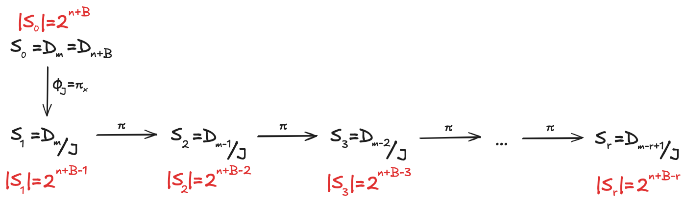
with degree $N=2^n$, blow-up factor $2^B$ and domain $D$, size $|D|= 2^{B+n}$. In this setting, the codewords are defined over elements of the circle group and correspond to special polynomials from a Riemann–Roch space (the bivariate polynomial space $\mathcal{L}_{N}(F)$ we define above).

Given a proximity parameter $\theta \in \left(0 , 1-\sqrt\rho \right)$, the goal is to prove that a function $f : X \to \mathbb{F}^D$ for representing the committed vector is $\theta$-close to a valid circle codeword in $\mathcal{C}$

Domain used in Circle FRI

The domain used in Circle FRI is just same as domain used in Circle FFT

Figure 15: Sequence of domain used in Circle FRI

Protocol

Circle FRI has two phases: Commit phase and Query phase

Commit phase

Before 1-st round, Prover needs to decompose $f \in \mathcal{L}_N(F)$ into $f = g + \lambda.v_n \ (\lambda \in F)$. This can be done by using vector projection and makes sure that $g \in \mathcal{L}'_N(F)$

Figure 16: Prover decomposes f and send unique lambda value to verifier

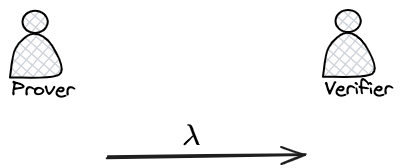
Prover have commited to $f$ ahead over domain $D_{n+B}$

Round 1:

Now we start folding process, the "even-odd" decomposition follows the same progression as in Circle FFT. In the 1-st round, we set $g_0 = g$ and write $g_0 = g_{0,0}(x) + y \cdot g_{0,1}(x)$

$$\begin{cases} g_{0,0}(x) = \frac{g_{0}(x,y) + g_{0}(x, -y)}{2} \\ g_{0,1}(x) = \frac{g_{0}(x,y) - g_{0}(x, -y)}{2y} \end{cases}$$

The prover receives a random challenge $\alpha_1$ from verifier and uses it to build a random linear combination: $g_1(x) = g_{0,0}(x) + \alpha_1.g_{0,1}(x)$. Then evaluate $g_1$ over $S_1$ and commit these evaluations using merkle commitment.

Round 2:

In 2^nd^ round, the prover continues decomposing $g_1(x) = g_{1,0}(\pi(x)) + x \cdot g_{1,1}(\pi(x))$ with:

$$\begin{cases} g_{1,0}(\pi(x)) = \frac{g_{1}(x) + g_{1}(-x)}{2} \\ g_{1,1}(\pi(x)) = \frac{g_{1}(x) - g_{1}(-x)}{2x} \end{cases}$$

Uses random challenge $\alpha_2$ receiving from Verifier, Prover build random linear combination: $g_2(x) = g_{1,0}(x) + \alpha_2.g_{1,1}(x)$ and commits $g_2$ over $S_2$.

... ... ...

Round r: ($r \le n+1$) at round r, the degree of polynomial is $2^{n-r}$ and if we think this degree is small enough for us then stop at this round. If $r = n+1$ then the final polynomial only have degree 0.

Generally in the r-th round, the prover holds a function $g_{r-1}$ from previous round. It calculate 2 polynomials $g_{r-1,0}(\pi(x))$ and $g_{r-1,1}(\pi(x))$ as:

$$\begin{cases} g_{r-1,0}(\pi(x)) = \frac{g_{r-1}(x) + g_{r-1}(-x)}{2} \\ g_{r-1,1}(\pi(x)) = \frac{g_{r-1}(x) - g_{r-1}(-x)}{2x} \end{cases}$$

It receives a random challenge $\alpha_r$, uses it to build random linear combination: $g_{r-1}(x) = g_{r-1,0}(x) + \alpha_{r}.g_{r-1,1}(x)$. Prover sends $g_r(x)$ in plain to verifier in the final round.

Figure 17: Visualization of commit phase

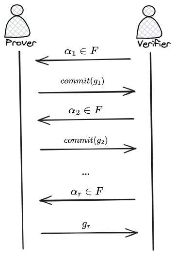
Query phase

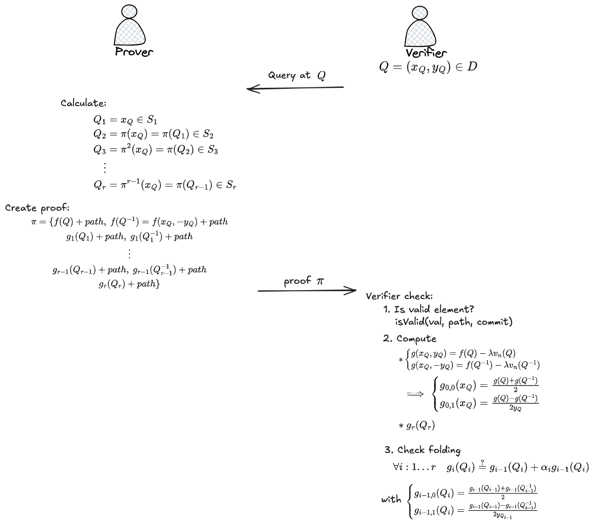
The verifier samples $s \geq 1$ queries uniformly from domain $D$. For each query $Q$, the verifier constructs a trace - a sequence of points generated by iteratively applying the squaring map together with the transformations specified by the protocol.

Starting from the initial point $Q_0 = Q = (x_Q,y_Q)$ these transformations are applied across multiple rounds, producing points $Q_j \in S_j, \quad j = 1..r$ where $S_j$ denotes the evaluation domain corresponding to the $j$-th round.

We denote $Q^{-1}$ as $J(Q)$, inverse of Q.

The verifier asks the prover for the values of:

• $f$ at $Q_0$ and $Q_{0}^{-1}$
• $g_1$ at $Q_1$ and $Q_{1}^{-1}$
• $g_2$ at $Q_2$ and $Q_{2}^{-1}$ ...
• $g_{r-1}$ at $Q_{r-1}$ and $Q_{r-1}^{-1}$

Beside values, Prover must provide merkle path to convince verifier about the authorize of these values.

From the values of $f$ at $Q_0$ and $Q_{0}^{-1}$, Verifier can calculate the value of $g$ at these points:

$$\begin{cases} g(Q_0) = f(Q_0) - \lambda v_{n}(Q_0) \\ g(Q_0^{-1}) = f(Q_0^{-1}) - \lambda v_{n}(Q_0^{-1}) \end{cases}$$

Verifier can also comput $g_r(Q_r)$ because $g_r$ is given to Verifier in plain.

From these values, verifier does the following checks:

$$\boxed{ \forall i \in \{1,...,r\} : g_i(Q_i) == g_{i-1}(Q_{i}) + \alpha_i g_{i-1}(Q_{i}^{-1})} \tag{*}$$

with:

• $g_{i-1}(Q_{i}) = \frac{g_{i-1}(Q_{i-1}) + g_{i-1}(Q_{i-1}^{-1})}{2}$
• $g_{i-1}(Q_{i}^{-1}) = \frac{g_{i-1}(Q_{i-1}) - g_{i-1}(Q_{i-1}^{-1})}{2 y_{Q_{i-1}}}$

In summary, Verifier does 3 things:

1. Check valid merkle proof for each value recieved from prover
2. Compute:
   • $g(Q_0)$, $g(Q_0^{-1})$
   • For all $i = 1..r$ :$g_{i-1}(Q_{i})$, $g_{i-1}(Q_{i}^{-1})$
   • $g_r(Q_r)$
3. Validate the equations (*).

The FRI protocol is demonstrate in figure 18:

Figure 18: Visualization of query phase

Circle STARK protocol

We now integrate all materials we explored above to form a complete Circle STARK protocol. The flow of Circle STARKs is represent in Section Flow of Circle STARKs.

Instead of doing directly Circle FRI over Composition Polynomial, it use DEEP Quotienting and then use Circle FRI to increase soundness of protocol.

Algebraic Intermediate Representation (AIR)

• Trace Domain: $H \subseteq C(F_p)$ is the standard position coset of size $N = 2^n$

• Trace values: $t_1,...,t_w \in F^{N}_p$ (Think of each trace as the values of a single register in a computer, recorded at every step from time 1 (start) to time N (end).)

• Interpolate:

$$\begin{array}{c|c} H & t_1 & t_2 &\cdots & t_w\\ \hline w_0 = (x_0, y_0) & t^{(0)}_{1} & t^{(0)}_{2} & \cdots & t^{(0)}_{w} \\ \vdots & \vdots & \vdots & \ddots & \vdots \\ w_{N-1} = (x_{N-1}, y_{N-1})& t^{(N-1)}_1 & t^{(N-1)}_2 & \cdots & t^{(N-1)}_w \\ & \downarrow & \downarrow & \cdots & \downarrow \\ & p_1 & p_2 & \cdots & p_w \end{array}$$

Use Circle FFT to interpolate each Trace column $t_i$ into bivarate polynomial $p_i(x,y)$ with:

$$p_i(x,y) = [c_0, \cdots, c_{N-1}] = c_0b_0(x,y) \ + \ \cdots \ + c_{N-1}b_{N-1}(x,y)$$

We have: $p_1, \cdots, p_w \in \mathcal{L}'_{N}(F_p)$

• Apply constraint: (assume we only consider constraint apply on 2 neighbouring row)
  • row $i$: $p_1(x_{i-1}, y_{i-1}),...,p_w(x_{i-1}, y_{i-1})$
  • row $i+1$: $p_1(x_i, y_i),...,p_w(x_i, y_i)$

Our constraint in general is something like:

$$P_j(s_j, p_1(x_{i-1}, y_{i-1}),\cdots,p_w(x_{i-1}, y_{i-1}), p_1(x_{i}, y_{i})\cdots,p_w(x_{i}, y_{i}))=0$$

With $s_j$ is the selector, but don't concern about it now. Think we have the set of defined constraints then selector is the way to choose which constraint will be apply for rows ${i, i+1}$.

Assume after apply all constraints that force the trace follow the logic of the execution we have $c$ constraint polynomials:

$$P_1, P_2, ...,P_c \in \mathcal{L}_{d \cdot N}(F_p)$$

with $d = max(deg(P_1), ... deg(P_c))$ and $deg(P_j) \leq \frac{p^2 + 1}{N} - 1$ with $p$ is CFFT-friendly prime (Mersenne31 prime in our case).

Why $deg(P_j) \leq \frac{p^2 + 1}{N} - 1$ is hard to understand and we don't understand too =D Please read the Circle STARKs paper for this point, but it does not important now, we just need to understand that $d$ is a constant bound for degree of bivariate polynomial $P_j$ (i.e., $P_j \in \mathcal{L}_{d \cdot N}(F_p)$ ).

One note for readers: in the Circle STARKs flow shown in Figure 1, after applying the constraints we obtain the Constraint Polynomials, and then we use the polynomial-quotient technique to convert these Constraint Polynomials into Quotient Polynomials—polynomials of the form $q(x)=0$.

In this section, we combine those two steps into one: the polynomials $P_j$ are already the Quotient Polynomials (since they are of the form $q(x)=0$).

Interactive Oracle Proof for AIR

In this section we denote $F$ as extension field of $\mathbb{F}_p$ that secure enough to draw random in it. For example, if our prime field $\mathbb{F}_p$ is Mersenne31 prime field with 32 bit, then to achieve 128-bit security we need choose $F$ as quadratic extension field of $\mathbb{F}_p$ (i.e., $\mathbb{F}_{p^4}$).

After deriving the Trace Polynomials and the Constraint (or Quotient) Polynomials, we do not directly verify whether the execution is correct. Instead, we check whether the Trace Polynomials $p_1,\dots,p_w$ cause the Constraint Polynomials $P_1,\dots,P_c$ to hold over the trace domain $H$.

And we use an Interactive Oracle Proof (IOP) to check this statement. The IOP for AIR consists of three steps:

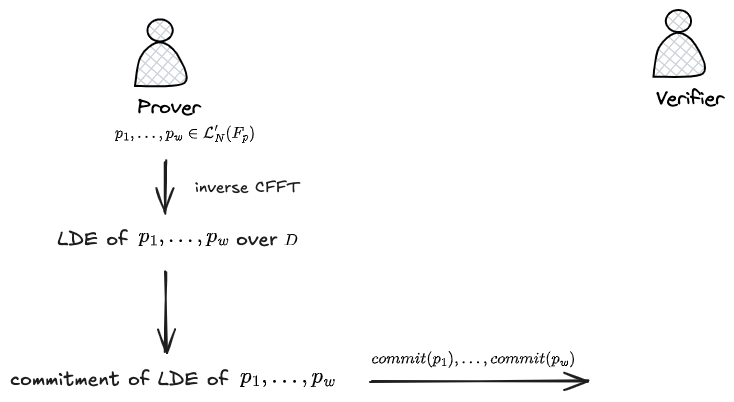
• Step 1: (LDE & commit Trace Polynomials) The prover uses an inverse Circle FFT to compute the low-degree extension (LDE) of $p_1,\dots,p_w$ over the evaluation domain $D$, where $\frac{|D|}{|H|} = 2^{B}$ (i.e., $D$ is $2^{B}$ times larger than $H$).

  The prover then sends the Merkle commitment of these LDEs to the verifier.

Figure 19: Step 1 in IOP for AIR

• Step 2: (Create Composition Polynomial & Decompose it) The verifier sends random challenges to the prover, who uses them to combine the Constraint Polynomials $P_1,\dots,P_c$ into a single Composition Polynomial (CP).

Figure 20: Step 2 in IOP for AIR

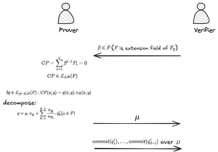
Instead of running FRI on the composition polynomial as in a traditional STARK, Circle STARKs use a technique called DEEP (Domain Extension for Eliminating Pretenders) to ensure that the composition polynomial is genuinely derived from the trace polynomials. In this technique, the prover decomposes

$$CP \;\longrightarrow\; q \;\longrightarrow\; q'_k \in \mathcal{L}_N(F)$$

where each $H_k$ is a twin-coset of size $|H_k| = N$ and $\overline{H} = \bigcup_{k=1}^{d-1} H_k$.

The prover then commits to the polynomial $q'_k$ (see Figure 20). This decomposition into $q'_k$ allows us to work with polynomials in $\mathcal{L}_N(F)$.

• Step 3: (Out-Of-Domain-Sample) The verifier samples a random point $\gamma$ outside both the trace domain $H$ and the evaluation domain $D$, and sends it to the prover. The prover evaluates the trace polynomials $p_1,\dots,p_w$ at $\gamma$ and at $g \bullet \gamma$ (where $g$ is the generator of $H$), as well as the polynomial $q'$ at $\gamma$, and returns these values to the verifier. Because our constraints is only on two consecutive rows then we only need 2 consecutive values $\gamma$ and $g \bullet \gamma$.

  The verifier then checks the two sides of the composition-polynomial equation:

  $$\sum_{j=1}^{c}\beta^{j-1} P_j \;=\; \bigl(\mu\,v_{\overline{H}} + \sum_{k=1}^{d-1} \frac{v_{\overline{H}}}{v_{H_k}}\,z_k \bigr) v_H .$$

Figure 21: Step 3 in IOP for AIR

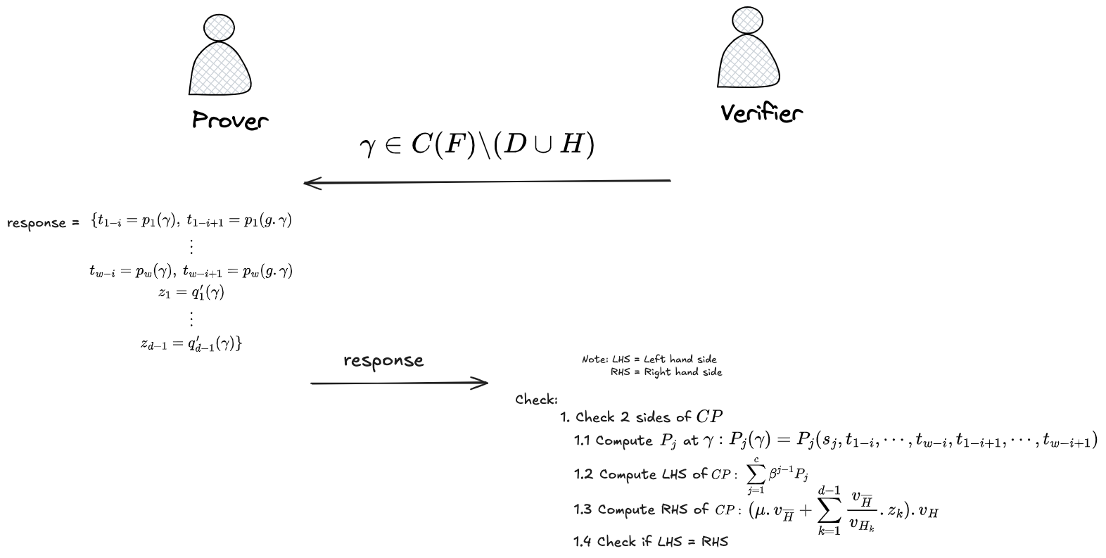
Verifier reject the overall Circle STARKs protocol if this check does not pass.

There is no Merkle “path” proof here because $\gamma$ and $g\gamma$ lie outside the committed domain $D$.

Low-degree Test

To ensure prover not to cheat about the value of $P_j$ and $q_j$ at $\gamma$ and $g \bullet \gamma$, we use the quotient trick:

DEEP Quotient

If $p_i(\gamma) = \tau$ then $\frac{p_i(x, y) - \tau}{v_{\gamma}(x, y)}$ is polynomial.

• Vanishing polynomial at point $\gamma = (\gamma_x, \gamma_y)$. $v_{\gamma}(x, y) = 1 - (\gamma_x.x + \gamma_y.y) - i.(-\gamma_y.x + \gamma_x.y)$. This bivariate polynomial evaluate to zero at only $\gamma = (\gamma_x, \gamma_y)$.

  This vanishing polynomial plays the same role as the familiar univariate vanishing polynomial $v_{\gamma}(x) = x - \gamma$ used for 1-dimensional points in the standard setting. The univariate $v_{\gamma}$ evaluates to zero at $x = \gamma$ and to a non-zero value everywhere else. In the bivariate case, constructing the vanishing polynomial is more involved than in the univariate case, but its purpose is identical: it evaluates to zero exactly on the specified point (or set of points) and remains non-zero elsewhere. You can verify this yourself. (But don't ask us why $v_{\gamma}(x, y)$ has this formulae, let ask the Circle STARKs authors =D)

• With $f \in \mathcal{L}_N(F)$ and every point $\gamma = (\gamma_x, \gamma_y)$ on circle curve. The single-point quotient: $q = \frac{f - f(\gamma)}{v_{\gamma}}$ in $\mathcal{L}_N(F(i))$. Because $v_{\gamma}$ have $i$ in it formulae then $q$ belong to $\mathcal{L}_N(F(i))$. If $F$ already have $i$ then $F(i) \equiv F$. We can decompose $q = \frac{f - f(\gamma)}{v_{\gamma}} = \mathsf{Re}(\frac{f-f(\gamma)}{v_{\gamma}}) + i.\mathsf{Im}(\frac{f-f(\gamma)}{v_{\gamma}})$ with $\mathsf{Re}(\frac{f-f(\gamma)}{v_{\gamma}})$ and $\mathsf{Im}(\frac{f-f(\gamma)}{v_{\gamma}})$ in $\mathcal{L}_N(F)$

  • $\mathsf{Re}(.)$ mean real part of complex "number"
  • $\mathsf{Im}(.)$ mean imagine part of complex "number"

• We create DEEP-quotient of $p_i$ and $q_j$ at $\gamma$ and $g.\gamma$

  $$\forall i = 1..w \\ \begin{cases} \frac{p_i - p_i(\gamma)}{v_{\gamma}} = \mathsf{Re}(\frac{p_i - p_i(\gamma)}{v_{\gamma}}) + i.\mathsf{Im}(\frac{p_i - p_i(\gamma)}{v_{\gamma}}) \\ \frac{p_i - p_i(g.\gamma)}{v_{g.\gamma}} = \mathsf{Re}(\frac{p_i - p_i(g.\gamma)}{v_{g.\gamma}}) + i.\mathsf{Im}(\frac{p_i - p_i(g.\gamma)}{v_{g.\gamma}}) \end{cases}$$ $$\forall j = 1..(d-1) : \frac{q_j - q_j(\gamma)}{v_{\gamma}} = \mathsf{Re}(\frac{q_j - q_j(\gamma)}{v_{\gamma}}) + i.\mathsf{Im}(\frac{q_j - q_j(\gamma)}{v_{\gamma}})$$

  with all $\mathsf{Re}(.)$ and $\mathsf{Im}(.)$ is in $\mathcal{L}_N(F)$

Now, Prover and Verifier engage in Circle FRI to check each $\mathsf{Re}(.)$ and $\mathsf{Im}(.)$ is low-degree polynomial in $\mathcal{L}_N(F)$ but they can do more efficiency by using linear combination and they need only 1 Circle FRI.

This mean Prover create a linear combination polynomial $\mathcal{F}$ from $\mathsf{Re}(.)$ and $\mathsf{Im}(.)$ with the random $\psi$ from Verifier:

$$\mathcal{F} = \sum_{i=1}^{w} \psi^i \cdot \mathsf{Re}(\frac{p_i - p_i(\gamma)}{v_{\gamma}}) + \sum_{i=1}^{d-1} \psi^{w+i} \cdot \mathsf{Re}(\frac{q_j - q_j(\gamma)}{v_{\gamma}}) + \sum_{i=1}^{w} \psi^{w+d-1+i} \cdot \mathsf{Im}(\frac{p_i - p_i(\gamma)}{v_{\gamma}}) + \sum_{i=1}^{d-1} \psi^{2w+d-1+i} \cdot \mathsf{Im}(\frac{q_j - q_j(\gamma)}{v_{\gamma}})$$

And then do only one Circle FRI to prove $\mathcal{F}$ is low-degree polynomial in $\mathcal{L}_N(F)$.

Verifier accept the overall Circle STARKs protocol if the Circle FRI protocol is accepted.

$$\text{-- CIRCLE STARKS PROTOCOL COMPLETED --}$$